[코드 리뷰] Contrastive Loss - InfoNCE(NT-Xent)

4 분 소요

code 다운로드: 📥 contrastive-loss.ipynb 다운로드

1. Introduction

“같은 것은 가까이, 다른 것은 멀리” 라는 아이디어에서 시작된 Contrastive learning은 Deep learning 분야에서 많이 각광 받아온 학습 방법이다.

Self-supervised learning 분야에서 주로 사용되며 2010년 말 빅테크기업에서 압도적인 연산력을 토대로 만들어낸 MoCo, SimCLR 같은 모델이 대표적인 예시이며, Multi-modal 학습 방법인 OpenAI의 CLIP의 C도 Contrastive이다.

Contrastive Loss는 여러가지가 있지만, 본 게시글에서는 SimCLR 논문에서 사용된 가장 많이 사용되는 Loss 중 하나인 InfoNCE 계열의 NT-Xent loss를 구현하고 코드 리뷰를 할 것이다.

Contrastive Loss에 대해 입문하거나 관심이 있다면 Understanding Contrastive Representation Learning through Alignment and Uniformity on the Hypersphere를 한번 읽어보는 것을 추천한다.

2. Preliminary

SimCLR은 2020년 구글에서 발표한 self-supervised learning 논문으로 한 sample에 두개의 augmented view를 만들어서 같은 이미지끼리는 큰 cosine similarity를 가지게 하고 서로 다른 이미지 샘플끼리는 낮은 cosine similarity를 가지도록 하는 방식으로 학습한다.

우선 수식부터 알아보자

\[\begin{equation} l(i, j)=-log\frac{exp(sim(z_i, z_j)/\tau)}{\sum^{2N}_{k=1} \mathbb{1}_{[k \neq i]}exp(sim(z_i, z_k)/\tau) } \end{equation}\]

위 식을 흐린눈 하고 보면 익숙한 수식이 보인다. 많은 블로거들이 외치듯 위 loss는 softmax의 형태를 하고 있다. 이 수식은 positive pair와 negative pair로 구분하도록 한다.

N은 batch size이다. 분모항의 sumation에서 2N이 나타난 이유는 모든 샘플에 있어서 2개의 augmented view를 생성하기 때문이다. 여기서 i와 j는 같은 sample의 서로 다른 augmented view이고 sim은 cosine similarity이다.

즉 i, j는 같은 sample이므로 positive pair가 되고 분모는 i가 자기 자신을 제외한 positive, negative pair의 cosine similarity를 지수승하여 합한 값이다.

$\tau$는 분포를 좀 더 뾰족하거나 완만하게 만들어준다.

implementation

참고 코드에서 class 내의 함수를 꺼내서 사용할 수 있도록 아주 약간 수정했으며 핵심 메커니즘은 그대로임을 미리 알린다.

import torch    
import torch.nn.functional as F

def NTXentLoss(features, batch_size, n_views, temperature, device):
    # classification 문제이기 때문에 labels을 생성함.
    labels = torch.cat([torch.arange(batch_size) for i in range(n_views)], dim=0)
    labels = (labels.unsqueeze(0) == labels.unsqueeze(1)).float()
    labels = labels.to(device)

    # cosine similarity를 global하게 계산함.
    features = F.normalize(features, dim=1) # 입력은 [B, D]
    similarity_matrix = torch.matmul(features, features.T)

    # discard the main diagonal from both: labels and similarities matrix 
    # diagonal 원소는 본인이기 때문에 k!=i를 지키기 위해 masking
    mask = torch.eye(labels.shape[0], dtype=torch.bool).to(device)
    
    # view 함수는 tensor 형태의 데이터의 shape을 바꿔주는 함수 - Shared Data / Memory Efficiency
    labels = labels[~mask].view(labels.shape[0], -1) # ~mask은 torch에서 True인 원소들을 없애고 값을 반환하므로 2N x (2N-1)짜리 행렬이 나오게 됨
    similarity_matrix = similarity_matrix[~mask].view(similarity_matrix.shape[0], -1)
    
    # 굳이 아래처럼 positives와 negatives를 일렬로 작업하는 이유는 cross entropy 계산 시 label을 항상 0번째 열로 고정할 수 있기 때문임.
    # select and combine multiple positives
    positives = similarity_matrix[labels.bool()].view(labels.shape[0], -1)

    # select only the negatives the negatives
    negatives = similarity_matrix[~labels.bool()].view(similarity_matrix.shape[0], -1)

    logits = torch.cat([positives, negatives], dim=1)
    labels = torch.zeros(logits.shape[0], dtype=torch.long).to(device)

    # temperature 계산
    logits = logits / temperature
    return logits, labels

BATCH_ZISE = N_VIEW = 2 # Batch가 2이고 augmentated view가 2개 있다고 가정했을 때

# labels 구성은 다음과 같다.
labels = torch.cat([torch.arange(BATCH_ZISE) for i in range(N_VIEW)], dim=0)
labels

tensor([0, 1, 0, 1])

# unsueeze는 추가하는 차원축의 인덱스를 지정할 수 있다.
print(labels.unsqueeze(0))
print(labels.unsqueeze(1))

tensor([[0, 1, 0, 1]])
tensor([[0],
        [1],
        [0],
        [1]])

labels = (labels.unsqueeze(0) == labels.unsqueeze(1)).float()
labels

tensor([[1., 0., 1., 0.],
        [0., 1., 0., 1.],
        [1., 0., 1., 0.],
        [0., 1., 0., 1.]])

# torch.eye는 대각 성분만 1이고 나머지는 0인 텐서를 만든다.
mask = torch.eye(labels.shape[0], dtype=torch.bool)
mask

tensor([[ True, False, False, False],
        [False,  True, False, False],
        [False, False,  True, False],
        [False, False, False,  True]])

# 마스킹을 하면 다음과 같이 True인 부분만 남기고 False인 부분은 없앤다. 이는 torch 특유의 연산이다.
m = torch.tensor([True, False])
l1 = torch.tensor([1,2])
l1[m]

tensor([1])

labels = labels[~mask].view(labels.shape[0], -1)
labels

tensor([[0., 1., 0.],
        [0., 0., 1.],
        [1., 0., 0.],
        [0., 1., 0.]])

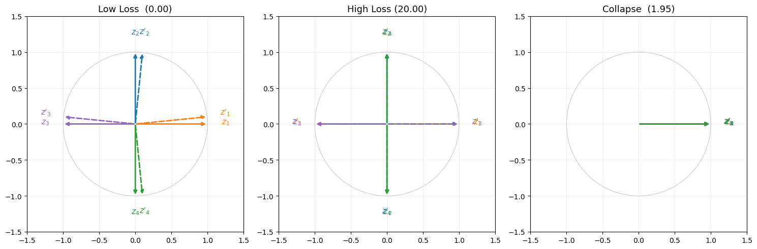
4. Low Loss, High Loss, Collapse Loss

이제 구현한 Loss를 활용하여 언제 Loss가 높아지고 낮아지는지 그리고 붕괴는 어떻게 일어나는지 알아보자.

import numpy as np
import matplotlib.pyplot as plt

# ── Low Loss ──────────────────────────────────────────────────────────────────
z1_low = torch.tensor([[1.0, 0.0], [0.0, 1.0], [-1.0, 0.0], [0.0, -1.0]])
z2_low = torch.tensor([[1.0, 0.1], [0.1, 1.0], [-1.0, 0.1], [0.1, -1.0]])  # z1이랑 거의 같은 방향

z = torch.cat([z1_low, z2_low], dim=0)
logits, labels = NTXentLoss(z, 4, 2, 0.1, 'cpu')
loss_low = F.cross_entropy(logits, labels).item()

print(f"Low  Loss: {loss_low:.4f}")

Low  Loss: 0.0003

# ── High Loss ─────────────────────────────────────────────────────────────────
z1_high = torch.tensor([[1.0, 0.0], [0.0, 1.0], [-1.0, 0.0], [0.0, -1.0]])
z2_high = torch.tensor([[-1.0, 0.0], [0.0, -1.0], [1.0, 0.0], [0.0, 1.0]])  # 정반대 방향

z = torch.cat([z1_high, z2_high], dim=0)
logits, labels = NTXentLoss(z, 4, 2, 0.1, 'cpu')
loss_high = F.cross_entropy(logits, labels).item()

print(f"High Loss: {loss_high:.4f}")

High Loss: 20.0002

Collapse란 model이 입력과 무관하게 상수의 값을 내뱉는 상황이다. Collapse가 일어나면 model의 representation이 저하된다. 따라서 InfoNCE는 큰 배치를 이용하여 분모를 키워 collapse penalty를 강하게 함으로써 collapse가 쉽게 일어나지 않도록 한다. 이것이 SimCLR이 대용량 배치(e.g. 4096)를 필요로 하는 이유이기도 하다.

# ── Collapse ─────────────────────────────────────────────────────────────────
z1_collapse = torch.tensor([[1.0, 0.0], [1.0, 0.0], [1.0, 0.0], [1.0, 0.0], ])
z2_collapse = torch.tensor([[1.0, 0.0], [1.0, 0.0], [1.0, 0.0], [1.0, 0.0], ])

z = torch.cat([z1_collapse, z2_collapse], dim=0)
logits, labels = NTXentLoss(z, 4, 2, 0.1, 'cpu')
loss_collapse = F.cross_entropy(logits, labels).item()

print(f"Collapse Loss: {loss_collapse:.4f}")

Collapse Loss: 1.9459

만능 클로드의 힘을 빌려 시각화를 하며 글을 마무리한다.

# ── 시각화 ────────────────────────────────────────────────────────────────────
COLORS = ['tab:orange', 'tab:blue', 'tab:purple', 'tab:green']
theta  = np.linspace(0, 2 * np.pi, 300)

fig, (ax1, ax2, ax3) = plt.subplots(1, 3, figsize=(15, 5))

for ax, title, loss_val, z1, z2 in [
    (ax1, f"Low Loss  ({loss_low:.2f})",      loss_low,      z1_low,      z2_low),
    (ax2, f"High Loss ({loss_high:.2f})",     loss_high,     z1_high,     z2_high),
    (ax3, f"Collapse  ({loss_collapse:.2f})", loss_collapse, z1_collapse, z2_collapse),
]:
    ax.plot(np.cos(theta), np.sin(theta), 'lightgray', lw=1)
    ax.set_aspect('equal')
    ax.set_xlim(-1.5, 1.5)
    ax.set_ylim(-1.5, 1.5)
    ax.set_title(title, fontsize=13)
    ax.grid(True, alpha=0.2)

    z1n = F.normalize(z1, dim=1).numpy()
    z2n = F.normalize(z2, dim=1).numpy()

    for i in range(4):
        c = COLORS[i]
        ax.annotate("", xy=z1n[i], xytext=(0,0),
                    arrowprops=dict(arrowstyle="-|>", color=c, lw=2))
        ax.annotate("", xy=z2n[i], xytext=(0,0),
                    arrowprops=dict(arrowstyle="-|>", color=c, lw=2, linestyle='dashed'))
        ax.text(*(z1n[i] * 1.25), f"$z_{i+1}$",  color=c, ha='center', fontsize=11)
        ax.text(*(z2n[i] * 1.25), f"$z'_{i+1}$", color=c, ha='center', fontsize=11)

plt.tight_layout()
plt.savefig("ntxent_circle.png")
plt.show()

Twitter Facebook LinkedIn

YSPARK

[코드 리뷰] Contrastive Loss - InfoNCE(NT-Xent)

1. Introduction

2. Preliminary

implementation

4. Low Loss, High Loss, Collapse Loss

공유하기

참고

[코드 리뷰] I-JEPA-(1) overall train code

[논문리뷰] Brain Network Transformer

[논문리뷰] Self-Supervised Learning from Images with a Joint-Embedding Predictive Architecture

[코드 리뷰] Tensor Slicing